Financial trading vs. asset optimization

What is financial trading?

Asset optimization and various branches of energy trading are often thought of as synonymous, interchangeable terms. While they do share certain characteristics and aspects of execution, they are not all one and the same thing. But let’s look at it layer by layer. Energy trading, at the most basic level, means one market participant has energy for sale, and a second market participant buys that energy for the going price at a particular point in time. This is where it gets complicated. The trading transaction described can differ in purpose and intention. When we talk about trading in the energy market, we can break it down into three different scenarios: financial trading, asset-backed financial trading, and asset optimization. What do they have in common, and how do they differ from each other?

Scenario 1: purely financial trade

A purely financial trade is the classic speculative approach we know from the stock exchange. The intention is to capitalize on market value without ever physically dispatching the traded commodity. In a financial trade, you sell third-party energy with the idea of buying it back cheaper and vice versa. Financial trades are typically assetless, meaning the buyer does not have an energy system available to extract power from. The primary goal is to exploit short-term price fluctuations in the market for profit rather than the physical generation or consumption of the energy sold at high and bought at low prices. For these reasons, financial trading is also referred to as proprietary or speculative trading. As a general rule, imbalances should be avoided because they can result in expensive balancing costs and penalties.

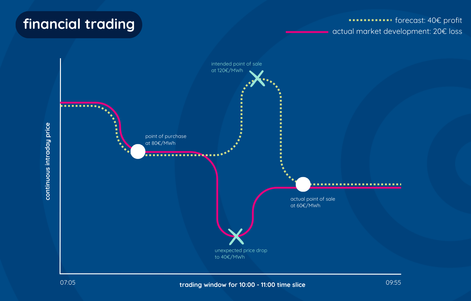
Graph 1: financial trading

This graph shows you a trading window for the 10-11:00 product in the continuous intraday market, from 7:05 to 9:55 in the morning. In this scenario, energy is bought for a price of 80€/MWh. The forecast predicts a price hike to 120€/MWh around the halfway mark, so this is where you plan to make your sale, yielding a 40€/MWh profit. However, it can happen that market conditions change suddenly; for example, due to weather events, outages, or technical errors. In this case, it leads to an unexpected price drop. As the trend evens out and joins back up with your forecast, you sell at 60€/MWh, incurring a loss of 20€/MWh on your original purchase.

Graph 1 is a simplified version of a real-life trading scenario. In actuality, an order known as stop-loss would get activated before you ever arrive at the 60€/MWh point. This mechanism exists to avoid unnecessary loss and is automatically triggered as soon as the market hits that pre-defined spot. The blue line in visual 2 illustrates the order activation at 70€/MWh, resulting in a 10€/MWh loss on the original purchase. Stop-loss also works in reverse, whereby you define the minimum amount you are willing to sell previously bought energy for.

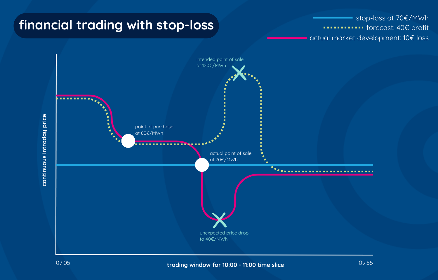
Graph 2: financial trading with stop-loss

Scenario 2: asset-backed financial trade

An asset-backed financial trade is similar to a purely financial trade in its intention to make money out of market value without delivery as the end goal. The difference is that the asset-backed variant has the support of a physical system to take energy from. If the market does not behave as expected, this asset acts as insurance against severe monetary loss. Again, such a situation occurs when prices increase after energy is sold with the intention of buying it back cheaper or when prices decrease after energy is bought with the intention of selling it at a higher price. To avoid making a loss, the seller activates the asset to physically deliver the energy volume in question.

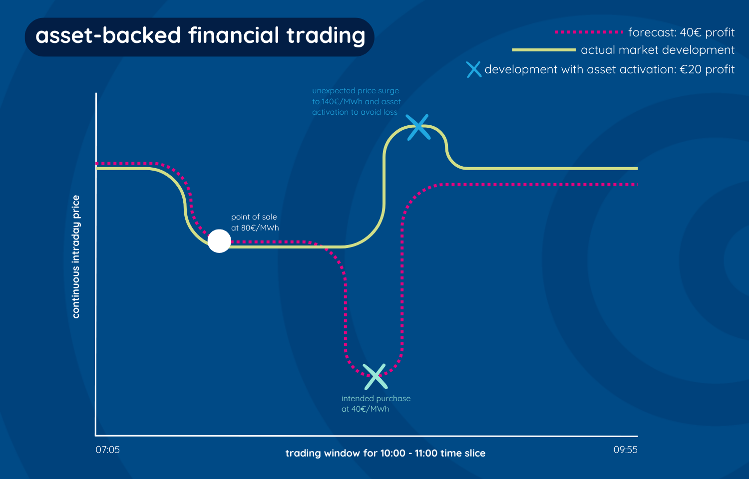
Graph 3: asset-backed financial trading

Graph 3 depicts the same situation as earlier. You sell energy at a price of 80€/MWh and intend to buy it back at the projected 40€/MWh price point. The market turns unexpectedly, and prices surge to 140€/MWh. Instead of risking a substantial loss, you decide to activate your asset and physically deliver the energy you sold. Assuming a marginal cost of 60€/MWh for your asset, that leaves you with a profit of 20€/MWh.

Scenario 3: asset optimization

Asset optimization is energy trading with the intention of physical execution. This type of trade aims to deliver sold energy and consume bought energy, at the same time respecting the asset’s physical limitations to ensure its longevity. To achieve good spreads, asset activities are aligned with favorable market conditions. For example, if you plan to charge a battery system in the early afternoon, but prices are uncharacteristically high that time of day, you can shift the charging schedule to a more opportune point in time. In contrast, discharging should occur during periods of high demand to maximize revenue.

That being said, financial trades still have a place in asset optimization. In this specific scenario, we refer to them as background trades. Not all the energy you trade is delivered or extracted on the spot. Financial trades are built around the (dis)charging processes to ensure maximum profitability and asset utilization. In the enspired trading world, we call this rebalancing. Forecast deviations are evaluated on a millisecond basis and readjusted according to the current market conditions. The term ‘rebalancing’ comes from the continuous re-optimization of the positions to achieve the commercial optimum without having to force a physical dispatch of the asset. Optimization is about making the asset perform ideally in the given market conditions. The trading transaction is attuned to the asset and not the other way around. Without automation, this would not be possible because the execution requires more analyses and higher reactivity than humans can process.

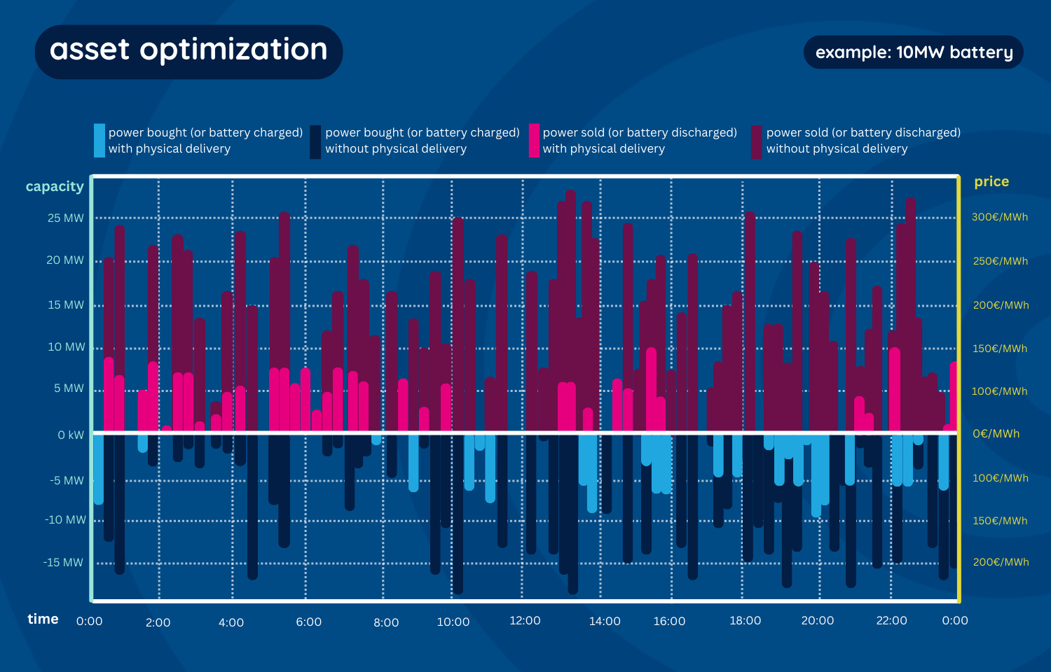
Graph 4: asset optimization

In graph 4, you can see an example of a 24-hour trading window for a 10 MW battery asset. The dark bars show the rebalancing activities, or in other words, how many trades occur without physical delivery or consumption. These trades can extend beyond the asset capacity and entail revenue stacking, which means the same product is sold or bought multiple times to maximize the profit from short-term price movements. Years of market experience have proven that asset optimization brings the most profitable and secure results. Beyond stable returns and minimal risk, it entails the added value of grid support and sustainable energy growth. In 2023, 2/3 of the revenue generated by the battery assets in our portfolio came from wholesale marketing and rebalancing.

How energy is traded: an overview

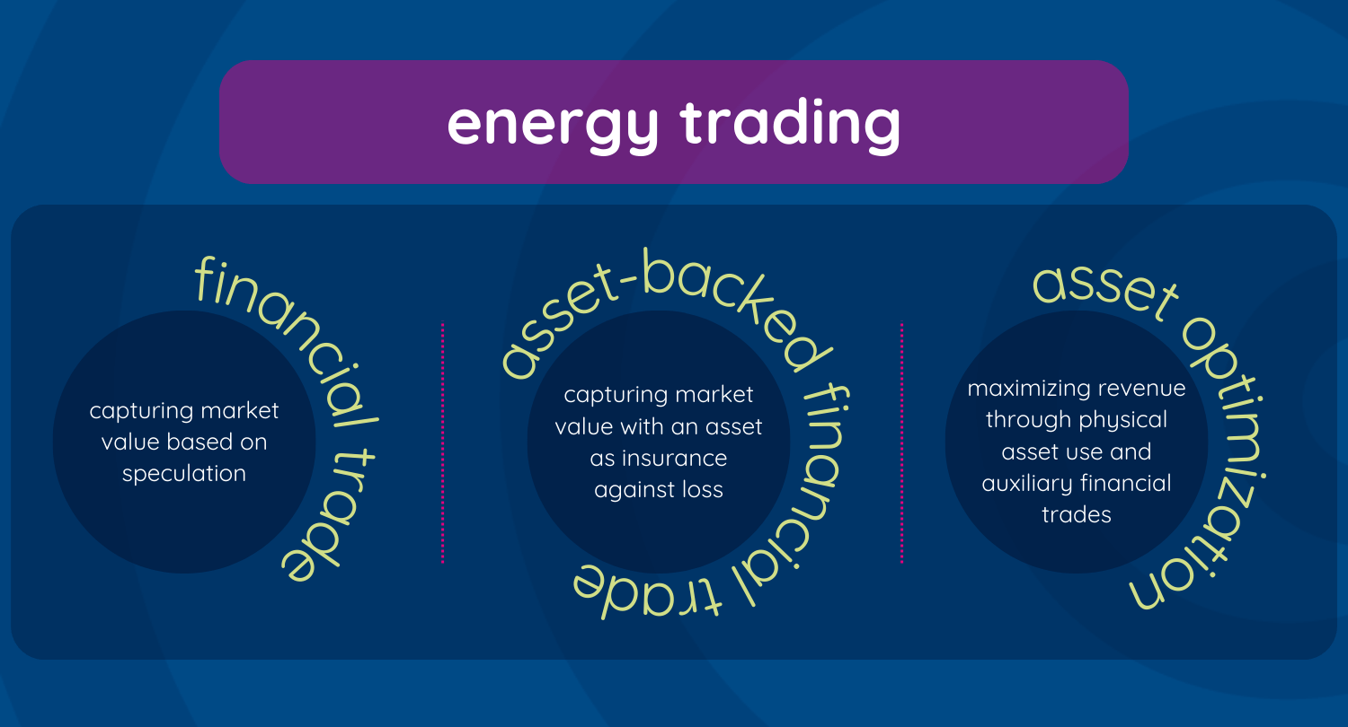
In conclusion, we differentiate between three trading scenarios. In a financial trade, market value is captured purely on the basis of speculation. In an asset-backed financial trade, you also capture market value based on speculation, but you can fall back on a physical energy system to mitigate loss incurrence. Asset optimization aims to maximize revenue by leveraging price volatility between the strategic physical activation points, all the while staying within technical limitations.

Graph 5: trading overview